Using GPU resources🔗

Many computational problems can be greatly sped up by using GPU resources, in many cases by a factor of 10 or more. Broadly speaking, this is particularly true for operations which are performed over large arrays, where the entire operation or some parts of it are local to some part of the array. Typical examples include elementwise arithmetic, matrix multiplication, integral calculus, tensor arithmetic, etc. NVIDIA provides an API, CUDA, which allows users to relatively easily write scientific computing code for GPU:s in a C-like programming environment. There are also libraries for CUDA, such as cuTensor, cuSparse, and cuBLAS, which provide access to tensor algebra, linear algebra and sparse linear algebra, respectively. Moreover, there are many libraries which leverage CUDA to provide GPU access through higher-level programming languages, such as Python.

CuPy🔗

CuPy is a Python package which provides CUDA wrappers for many functions in Numpy and SciPy. It allows for very easy porting of code written in Numpy and SciPy, and allows access to cuTensor, cuBLAS and cuSparse, often by simply replacing import numpy as np with import cupy as np.

The following examples were run on Vera nodes with 8 CPU:s in a Jupyter notebook, with the modules CuPy, matplotlib and IPython loaded. We will show tests with A40 and T4 GPU:s. Note that if your calculations particularly depend on using float64, you may be best off using V100 or A100 GPU:s.

Example: Matrix multiplication and reduction in NumPy and CuPy🔗

import numpy as np
import cupy as cp
from timeit import timeit

dtype = np.float32
m, k, n = (10000, 5000, 7000)
# These matrices are quite large, needing about 800 MB RAM
r = np.random.default_rng(987654321)
matrix_1 = r.random(size=(m, k), dtype=dtype)
matrix_2 = r.random(size=(k, n), dtype=dtype)
result_matrix_cpu = np.zeros((n), dtype=dtype)
temp_cpu = np.zeros((m, n), dtype=dtype)

# `cp.array` will copy the matrices to the GPU.
matrix_1_gpu = cp.array(matrix_1, dtype=dtype)
matrix_2_gpu = cp.array(matrix_2, dtype=dtype)
temp_gpu = cp.zeros((m, n), dtype=dtype)
result_matrix_gpu = np.zeros_like(result_matrix_cpu, dtype=dtype)

# Small functions for testing
def cpu_test_1():
    for i in range(10):
        np.matmul(matrix_1, matrix_2, out=temp_cpu)
        np.sum(temp_cpu, axis=0, out=result_matrix_cpu)

def cpu_test_2():
    for i in range(10):
        np.einsum('ij,jk->...k', matrix_1, matrix_2, out=result_matrix_cpu, optimize='optimal')

# To avoid over-syncing, we put the .get() outside the loop.
def gpu_test_1():
    for i in range(10):
        cp.matmul(matrix_1_gpu, matrix_2_gpu, out=temp_gpu)
    result_matrix_gpu[...] = cp.sum(temp_gpu, axis=0).get()

def gpu_test_2():
    for i in range(10):
        temp = cp.einsum('ij,jk->...k', matrix_1_gpu, matrix_2_gpu)
    result_matrix_gpu[...] = temp.get()

# We test with 3 iterations. Note that we run each function once before testing.
# For CuPy, the first function call is typically much slower than subsequent ones.
time_cpu_1 = timeit(cpu_test_1, setup=cpu_test_1, number=1)
time_gpu_1 = timeit(gpu_test_1, setup=gpu_test_1, number=1)

# Print results.
print(f'Data type: {matrix_1.dtype}\n'
      '---------------------------------------------\n')

print('====TEST MATMUL -> SUM====\n'
      '==========================\n'
      f'CPU time: {time_cpu_1:.4f}\n'
      f'GPU time: {time_gpu_1:.4f}\n'
      f'Speedup: {time_cpu_1 / time_gpu_1:.2f}\n'
      '==========================\n')
check_elements = np.allclose(result_matrix_cpu, result_matrix_gpu, atol=1e-8, rtol=1e-8)
check_elements_looser = np.allclose(result_matrix_cpu, result_matrix_gpu, atol=1e-4, rtol=1e-4)

print(f'All elements within allowance of 1e-8: {check_elements}')
print(f'All elements within allowance of 1e-4: {check_elements_looser}\n')
if m*k*n < 1e10:
    time_cpu_2 = timeit(cpu_test_2, setup=cpu_test_2, number=1)
else:
    time_cpu_2 = np.inf
time_gpu_2 = timeit(gpu_test_2, setup=gpu_test_2, number=1)

# Print results.
print('=======TEST EINSUM========\n'
      '==========================\n'
      f'CPU time: {time_cpu_2:.4f}\n'
      f'GPU time: {time_gpu_2:.4f}\n'
      f'Speedup: {time_cpu_2 / time_gpu_2:.2f}\n'
      '===========================\n')
check_elements = np.allclose(result_matrix_cpu, result_matrix_gpu, atol=1e-8, rtol=1e-8)
check_elements_looser = np.allclose(result_matrix_cpu, result_matrix_gpu, atol=1e-4, rtol=1e-4)

print(f'All elements within allowance of 1e-8: {check_elements}')
print(f'All elements within allowance of 1e-4: {check_elements_looser}\n')

cpu_best = min(time_cpu_1, time_cpu_2)
gpu_best = min(time_gpu_1, time_gpu_2)
print('=======BEST TIMES========\n'
      '==========================\n'
      f'CPU time: {cpu_best:.4f}\n'
      f'GPU time: {gpu_best:.4f}\n'
      f'Speedup: {cpu_best / gpu_best:.2f}\n'
      '==========================\n')

# Check that all elements are close. Note that we use the `get` method of the CuPy array
# in order to copy it from the GPU into host RAM.
print('--------------------------------------------\n')

Results for A40 GPU:🔗

>>> Data type: float32
>>> ---------------------------------------------
>>> 
>>> ====TEST MATMUL -> SUM====
>>> ==========================
>>> CPU time: 5.4996
>>> GPU time: 0.3111
>>> Speedup: 17.68
>>> ==========================
>>> 
>>> All elements within allowance of 1e-8: False
>>> All elements within allowance of 1e-4: True
>>> 
>>> =======TEST EINSUM========
>>> ==========================
>>> CPU time: inf
>>> GPU time: 0.0168
>>> Speedup: inf
>>> ===========================
>>> 
>>> All elements within allowance of 1e-8: False
>>> All elements within allowance of 1e-4: True
>>> 
>>> =======BEST TIMES========
>>> ==========================
>>> CPU time: 5.4996
>>> GPU time: 0.0168
>>> Speedup: 327.41
>>> ==========================
>>> 
>>> --------------------------------------------
>>> --------------------------------------------
>>> 
>>> Data type: float64
>>> ---------------------------------------------
>>> 
>>> ====TEST MATMUL -> SUM====
>>> ==========================
>>> CPU time: 10.1334
>>> GPU time: 14.1453
>>> Speedup: 0.72
>>> ==========================
>>> 
>>> All elements within allowance of 1e-8: True
>>> All elements within allowance of 1e-4: True
>>> 
>>> =======TEST EINSUM========
>>> ==========================
>>> CPU time: inf
>>> GPU time: 0.0289
>>> Speedup: inf
>>> ===========================
>>> 
>>> All elements within allowance of 1e-8: True
>>> All elements within allowance of 1e-4: True
>>> 
>>> =======BEST TIMES========
>>> ==========================
>>> CPU time: 10.1334
>>> GPU time: 0.0289
>>> Speedup: 350.36
>>> ==========================
>>> 
>>> --------------------------------------------

Note that for the matrix multiplication test, the CuPy version is only faster in the case of the data type float32, and about the same for float64. On the other hand, NumPy refuses to parallelize this particular np.einsum paths (more restrictive paths which do not require reduction can be parallelized), which makes it nearly impossible to run with large matrices, whereas CuPy can compile it into a single CUDA kernel and thereby obtain a large speedup.

The get() method of CuPy arrays force synchronization at the end of each test, which penalizes CuPy somewhat - in a longer computation where most of it is done on the GPU, CuPy would see larger benefits.

Results for T4 GPU🔗

>>> Data type: float32
>>> ---------------------------------------------
>>> 
>>> ====TEST MATMUL -> SUM====
>>> ==========================
>>> CPU time: 6.5629
>>> GPU time: 1.6036
>>> Speedup: 4.09
>>> ==========================
>>> 
>>> All elements within allowance of 1e-8: False
>>> All elements within allowance of 1e-4: True
>>> 
>>> =======TEST EINSUM========
>>> ==========================
>>> CPU time: inf
>>> GPU time: 0.0417
>>> Speedup: inf
>>> ===========================
>>> 
>>> All elements within allowance of 1e-8: False
>>> All elements within allowance of 1e-4: True
>>> 
>>> =======BEST TIMES========
>>> ==========================
>>> CPU time: 6.5629
>>> GPU time: 0.0417
>>> Speedup: 157.38
>>> ==========================
>>> 
>>> --------------------------------------------
>>> --------------------------------------------
>>>
>>> Data type: float64
>>> --------------------------------------------
>>> 
>>> ====TEST MATMUL -> SUM====
>>> ==========================
>>> CPU time: 13.0603
>>> GPU time: 27.8300
>>> Speedup: 0.47
>>> ==========================
>>> 
>>> All elements within allowance of 1e-8: True
>>> All elements within allowance of 1e-4: True
>>> 
>>> =======TEST EINSUM========
>>> ==========================
>>> CPU time: inf
>>> GPU time: 0.0730
>>> Speedup: inf
>>> ===========================
>>> 
>>> All elements within allowance of 1e-8: True
>>> All elements within allowance of 1e-4: True
>>> 
>>> =======BEST TIMES========
>>> ==========================
>>> CPU time: 13.0603
>>> GPU time: 0.0730
>>> Speedup: 178.97
>>> ==========================
>>> 
>>> --------------------------------------------

The results for the T4 GPU are broadly similar, except the A40 is about 2 (for float64) to 5 (for float32) times as fast as the T4, which matches roughly with their stated capabilities on the hardware details page.

Example: Regularized least squares with sparse matrices🔗

This is a more complicated example, using a common type of optimization - ridge regression of a sparse matrix equation with $L_2$ regularization.

import cupyx.scipy.sparse as sp
import cupyx.scipy.sparse.linalg as splg
import numpy as np
from scipy.sparse import random as sparse_random
import cupy as cp
from time import time

r = np.random.default_rng(1234)
rows = 15000
columns = 15000
# We create a random system matrix with a density of 0.1 (thus, fairly dense)
system_matrix = sparse_random(m=columns, n=rows, density=0.1, dtype=np.float32, random_state=r)
system_matrix = sp.csr_matrix(system_matrix)

# We create random "data" using an normal distribution.
data = cp.array(r.normal(loc=3., scale=1., size=(rows, 1)))
extended_data = cp.vstack([data, cp.zeros((columns, 1))])

# Our solver, which will behave like an iterator.
def solve_reg_system(coeff_range, coeff_number):
    coeffs = np.geomspace(*coeff_range, coeff_number)
    for reg_coeff in coeffs:
        # Our regularization can represented by simply appending an identity matrix to the system matrix.
        reg_matrix = reg_coeff * sp.eye(rows, format="csr")
        reg_system_matrix = sp.vstack([system_matrix, reg_matrix])
        result = splg.lsmr(A=reg_system_matrix, b=extended_data)
        model = result[0][:rows]
        yield (reg_coeff, cp.linalg.norm(system_matrix @ model - data).get(),
               cp.linalg.norm(reg_matrix @ model).get() / reg_coeff)

wall_time = time()
# We hand the range of regularization coefficients to the solver.
solver = solve_reg_system((1e-1, 5e3), 10)
l_curve = np.array([t for t in solver])
coeff, residual, reg_norm = l_curve[:, 0], l_curve[:, 1], l_curve[:, 2]
wall_time = wall_time - time()
print(f'Wall time: {wall_time} s')

# A40
>>> Wall time: 2.54 s
# T4
>>> Wall time: 4.46 s

For comparison, running the nearly identical NumPy/SciPy code (replacing cp with np and removing the .get() methods) yields a wall time of around 90 s, for a speedup of about 20-40. This code is far from optimal for this problem, but the speedup is still substantial, although it will depend greatly on the parameters of the system matrix.

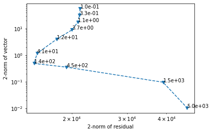
We plot the residual as a function of the regularization norm to get an "L-curve".

import matplotlib.pyplot as plt
fig, ax = plt.subplots()
ax.set_xscale('log')
ax.set_yscale('log')
ax.set_ylabel('2-norm of vector')
ax.set_xlabel('2-norm of residual')
ax.plot(residual, reg_norm, '--', marker='v')
for i, c in enumerate(coeff):
    ax.annotate(f'{c:.1e}', (residual[i], reg_norm[i])) 

CuPy is somewhat limited in its scope, focusing exclusively on replicating the functionality of these libraries. This means that it is not necessarily optimal in terms of performance, and it does not as of this writing provide any convenient tools for handling common limitations in GPU-based programming, such as running out of VRAM. It can be particularly ungracious when handling e.g. sparse matrix-dense vector multiplication, requesting copious amounts of VRAM rather than attempting to slice the problem.

However, it is very useful for speeding up already existing code, especially if the code is also modified to best leverage CuPy. In particular, as we have seen, across-the-board improvements are seen with float32 operations, but in cases where GPU hardware is most effectively utilized, float64 operations can also benefit greatly. Moreover, CuPy is one of the most convenient ways to use the cuTensor, cuBLAS, and cuSparse libraries.

Numba🔗

Numba provides the module numba.cuda for creating JIT (just-in-time) compiled functions which are parsed into CUDA. Much like the way standard Numba provides the opportunity to write Python code with performance comparable to that of C, numba.cuda allows you to write Python code which is parsed and compiled into CUDA kernels.

Generally, using Numba to write efficient code can require fairly advanced CUDA programming knowledge - this means paying attention to shared memory, array slicing, registers, and so forth. It is typically difficult to write code that is competetive with standard libraries for e.g. matrix multiplication, as we can see in this example of the same matrix-addition reduction which borrows some lightly optimized code from the Numba documentation:

Bad example: Matrix multiplication and reduction in Numba🔗

import numba.cuda as cuda
from numba import float32
import numpy as np
from timeit import timeit


m, k, n = (10000, 5000, 7000)
r = np.random.default_rng(987654321)
A = r.random(size=(m, k), dtype=np.float32)
B = r.random(size=(k, n), dtype=np.float32)
out = np.zeros((n), dtype=np.float32)

TPB = 16
threadsperblock =  (TPB, TPB)
blockspergrid = (int(np.ceil(A.shape[0] / (TPB))),
                 int(np.ceil(B.shape[1] / (TPB))))


@cuda.jit
def matmul_reduce(A, B, out):
    # Define an array in the shared memory
    # The size and type of the arrays must be known at compile time
    sA = cuda.shared.array(shape=(TPB, TPB), dtype=float32)
    sB = cuda.shared.array(shape=(TPB, TPB), dtype=float32)
    sC = cuda.shared.array(shape=(TPB, TPB), dtype=float32)
    x, y = cuda.grid(2)
    tx = cuda.threadIdx.x
    ty = cuda.threadIdx.y
    bpg = cuda.gridDim.x    # blocks per grid
    # Each thread computes one element in the result matrix.
    # The dot product is chunked into dot products of TPB-long vectors.
    tmp = 0.
    for i in range(bpg):
        # Preload data into shared memory

        if x <= A.shape[0] and ty + i * TPB <= A.shape[1]:
            sA[tx, ty] = A[x, ty + i * TPB]
        else:
            sA[tx, ty] = 0
        if tx + i * TPB <= B.shape[0] and y<= B.shape[1]:
            sB[tx, ty] = B[tx + i * TPB, y]
        else:
            sB[tx, ty] = 0
        # Wait until all threads finish preloading
        cuda.syncthreads()

        # Computes partial product on the shared memory
        for j in range(TPB):
            tmp += sA[tx, j] * sB[j, ty]

        # Wait until all threads finish computing
        cuda.syncthreads()

    sC[tx, ty] = tmp
    cuda.syncthreads()
    s = 1
    while s < TPB:
        if tx % (2 * s) == 0:
            # Stride by `s` and add
            sC[tx,ty] += sC[tx + s, ty]
        s *= 2
        cuda.syncthreads()

    # After the loop, the zeroth  element contains the sum
    if (tx == 0 and y < out.size):
        cuda.atomic.add(out, y, sC[tx, ty])

# Move arrays to device (GPU)
A_gpu = cuda.to_device(A)
B_gpu = cuda.to_device(B)
out_gpu = cuda.to_device(out)
ntimes = 3
def init_numba():
    matmul_reduce[blockspergrid, threadsperblock](A_gpu, B_gpu, cuda.device_array_like(out))
def test_numba():
    for i in range(ntimes):
        matmul_reduce[blockspergrid, threadsperblock](A_gpu, B_gpu, out_gpu)
    # Copy result back to host
    out[...] = out_gpu.copy_to_host()


time_gpu = timeit(test_numba, setup=init_numba, number=1)

print(f'Time: {time_gpu/ntimes:.2f}')

On an A40 GPU:

>>> Time: 7.26

This is not competetive with even NumPy, let alone CuPy. In fact, writing code to be competetive with the cuBLAS and cuTensor libraries requires many, many layers of optimization, as described in this excellent illustrated blog post. For this reason, it is always best to check if there are standard libraries in CUDA that perform similar functions before attempting to write a kernel.

Numba can interact with CuPy; a cupy.ndarray can be used directly by a Numba kernel with no need for wrapping. Thus, it is best to use cupy for linear algebra and tensor operations, and Numba for more general CUDA programming, as Numba does not have any bindings to CUDA linear algebra or tensor libraries.

Good example: 2D diffusion🔗

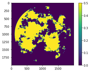
A good example of a relatively simple CUDA kernel that performs well is a diffusion kernel. First, we generate a jagged image:

import numpy as np
from numpy import fft

j, k = (2000, 2000)
r = np.random.default_rng(3966789)
field = r.random(size=(j, k), dtype=np.float32)
field = fft.fftshift(fft.fft2(field))
radius = 1 + np.sqrt((np.arange(j).reshape(-1, 1) - j // 2) ** 2 + (np.arange(k).reshape(1, -1) - k // 2) ** 2)
field = field * (radius ** -1.7)
field = fft.ifft2(fft.ifftshift(field)) * (radius < 0.45 * j)
field = field.real * (field.real > np.percentile(field.real, 70))

Then we write a kernel which loads each block, plus extra rows and columns at the edges, into shared memory, and calculates the two-dimensional discrete laplacian. It outputs the laplacian (which we suppose we might want to know at any given time), and moves the diffusion forward by one step, determined by a coefficient.

from numba import float32
import numba.cuda as cuda
TPB = 8
threadsperblock =  (TPB, TPB)
blockspergrid = (int(np.ceil(field.shape[0] / (TPB))),
                 int(np.ceil(field.shape[1] / (TPB))))
# Compile-time constants.
shasize = TPB + 2
coeff = 0.25
@cuda.jit
def diffusion(field, lapl):
    x, y = cuda.grid(2)
    # Shared array has two extra rows and columns to store edge values
    sharedarray = cuda.shared.array(shape=(shasize, shasize), dtype=float32)
    tx = cuda.threadIdx.x
    ty = cuda.threadIdx.y
    # Don't try to load edge values from outside the array
    if tx == 0 and x > 0:
        sharedarray[0, ty + 1] = field[x - 1, y]
    if ty == 0 and y > 0:
        sharedarray[tx + 1, 0] = field[x, y - 1]
    if tx == TPB - 1 and x < field.shape[0] - 1:
        sharedarray[-1, ty + 1] = field[x + 1, y]
    if ty == TPB - 1 and y < field.shape[1] - 1:
        sharedarray[tx + 1, -1] = field[x, y + 1]
    # Load all inner values into tx + 1, ty + 1.
    sharedarray[tx + 1, ty + 1] = field[x, y]
    val = 4 * sharedarray[tx + 1, ty + 1]
    # Synchronize after loading
    cuda.syncthreads()
    # Check that we are not at the very edges of the array before applying laplacian.
    if x > 0:
        val -= sharedarray[tx, ty + 1]
    if y > 0:
        val -= sharedarray[tx + 1, ty]
    if x < field.shape[0] - 1:
        val -= sharedarray[tx + 2, ty + 1]
    if y < field.shape[1] - 1:
        val -= sharedarray[tx + 1, ty + 2]
    # Check that we are within boundaries when saving laplacian and applying result in-place.
    if x < field.shape[0] and y < field.shape[1]:
        lapl[x, y] = val
        field[x, y] -= val * coeff

Suppose we want to iterate this 10000 times. How long will it take on an A40 GPU?

orig_field = field.copy()
field_gpu = cuda.to_device(field)
lapl = np.zeros_like(field)
lapl_gpu = cuda.to_device(lapl)
ntimes = 10000
def init_numba():
    diffusion[blockspergrid, threadsperblock](field_gpu, lapl_gpu)
def test_numba():
    for i in range(ntimes):
        diffusion[blockspergrid, threadsperblock](field_gpu, lapl_gpu)
    lapl[...] = lapl_gpu.copy_to_host()
    field[...] = field_gpu.copy_to_host()
time_gpu = timeit(test_numba, setup=init_numba, number=1)
print(f'Time per iteration: {time_gpu / ntimes}')

import matplotlib.pyplot as plt
f, ax = plt.subplots(1, 3, figsize=(12, 3.5))
im1 = ax[0].imshow(orig_field)
ax[0].set_title('Original image')
im2 = ax[1].imshow(field)
ax[1].set_title('10000 iterations')
im3 = ax[2].imshow(lapl, cmap='inferno', vmin=np.percentile(lapl, 5), vmax=np.percentile(lapl, 95))
ax[2].set_title('Laplacian')

>>> Time per iteration: 0.000272

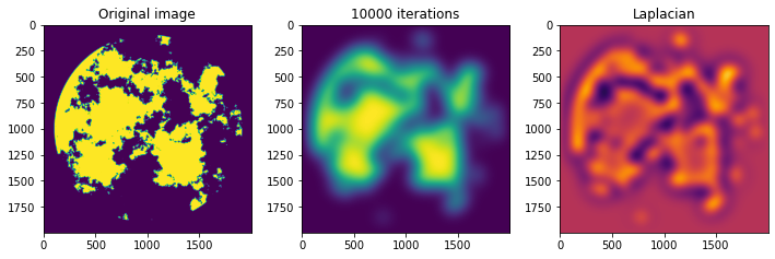
In the end, 10000 diffusion iterations took us only about 2.7 seconds! If we suppose that we do not care about knowing the laplacian after every invocation, the time goes down to 2.4 seconds. This type of problem, that can be broken down into repeated action on a localized part of an array, is a typical case where a GPU implementation can be relatively easy to draft.